Heatlh Insurance Analysis
Collorated work with Jin Choi, Shih-Lun Huang, Wei-Han Hsu
Click HERE to get the data source
Click HERE to see the full and detailed script
Project Overview
- Conduct power analysis and hypothesis testing to identify any relationship between the premium price and age, surgery history, existence of diabetes, and chronic disease history.
- Compare LASSO regression, Ridge regression, and Elastic net regression to identify the regularized regression model that will perform the best to predict the premium price for the health insurance data.
- Perform Principal Component Analysis (PCA), K-Mean’s clustering and XGBoost classifier to create the decision tree to determine one’s diabetes status.
1. Introduction
In the domain of health insurance, a variety of factors influence a customer’s premium price (cost of insurance), and the process of setting premium prices is typically carried out by the pricing and underwriting department. As data is more accessible and easily stored, the healthcare industry generates a large amount of data related to patients, diseases, and diagnoses, but this data has not been properly analyzed, leading to a lack of understanding of its significance and its potential impact on patient healthcare costs. Since there are several factors that can affect the cost of healthcare or insurance, it is important for a variety of stakeholders and health departments to accurately predict individual healthcare expenses using prediction models. The goal of this project is to properly analyze the patient’s data to design models to accurately predict the premium price and also observe significant characteristics of the data.
2. Data Preparation
The data was retrieved from Kaggle and has a total dimension of 1000 rows and 11 columns. Each row represents a customer of the insurance, and each column represents various features that describe a customer. The features include: age, presence of diabetes, blood pressure issues, transplant history, chronic disease history, height, weight, known allergies, cancer in the family history, number of major surgeries, and the premium price. Fortunately, the data did not contain any missing values or null values, hence there was no need for handling any missing values. Upon using a box plot to observe any noticeable outliers, we could not detect any presence of outliers in the data. We normalized the non-categorical features for faster computation as well as easier comparison and interpretability. To eliminate any unnecessary features, we conducted LASSO regression, and it turned out that none of the coefficients turned out to be zero, thus we kept all features.
3. Inference
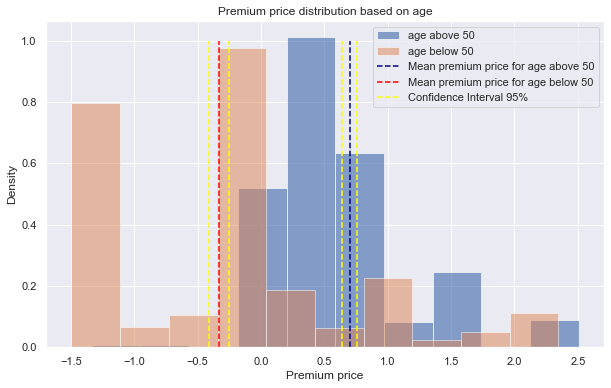
Parsed the data to create two distinct distributions per each of the four features based on the premium price. Then, we conducted the power analysis by setting the desired power to be 0.8, significance level to be .05, finding the effect size of the two distributions, and determining whether we have adequate sample sizes. Then, computed hypothesis testing using the Welch’s t-test since the variance between the two groups are different and that we compare scores between two different groups.
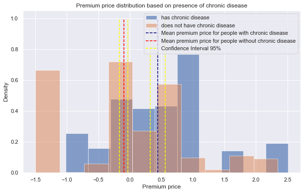
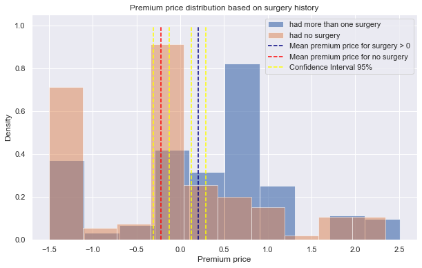
Looking at Figure 1, the mean premium price for the two distributions are far apart, without any overlaps of the confidence intervals. After conducting Welch’s t-test on distributions of ages above 50 and below 50, the p-value was 5.584x10-82. Since this value is smaller than the alpha value (.05), we reject the null hypothesis and conclude that age group has influence on the premium price. Similarly, the p-values for Welch’s t-test on distributions of presence of chronic disease (Figure 2) and surgery history (Figure 3) are 1.73x10⁻¹³, 1.6x10⁻¹¹, respectively. For either case, we reject the null hypothesis since the p-values are far less than the alpha level, thus we conclude that presence of chronic disease and surgery history are influential in the premium price.
 |
|---|
| Figure 1 |
 |
|---|
| Figure 2 |
 |
|---|
| Figure 3 |
4. Regression
We implemented regularized regression models to prevent the “curse of dimensionality” caused by the multivariate yet limited data set. Here, we built the three most popular ones: Lasso Regression, Ridge Regression, and Elastic Net. We then applied GridSearchCV, a type of cross-validation method, to fine-tune each model’s parameters. Alpha levels which were between 0.0001 and 20, were tested to find the optimal value.
 |
|---|
| Figure 4 |
 |
|---|
| Figure 5 |
 |
|---|
| Figure 6 |
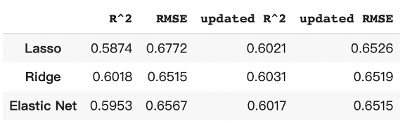
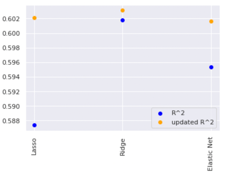
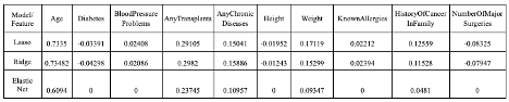
In Figure 6, the coefficient scores for “Age” indicate a high mathematical relationship with the target, “PremiumPrice”; As for “Height,” the scores tell us a low correlation with the target in all three models. The R2 value tells us that the predictor variables in the models are able to explain about 60% of the premium prices. The RMSE value means the average deviation between the predicted premium price made by the model and the actual price. To improve the model performance, we tried eliminating the variable “Height” since it has the lowest coefficient score. The R2 and RMSE comparison between the models “with Height” and “without Height” are shown in Figure 4 and Figure 5. The results tell us that there are slight improvements in all three models. Overall, ridge regression has the highest accuracy in predicting Premium Price.
5. Classification
In the previous parts, we explored the relationship between each feature and how to predict premium prices. In this part, we try to answer a different question. With all the given features in the datasets will we be able to determine a person’s diabetes status?
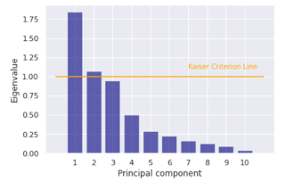
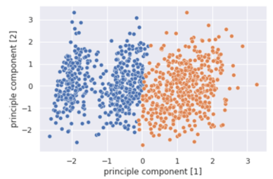
In order to better cluster the data, we implement principle component analysis to decrease the dimension of the data. First, we center the data by standardizing features with their means and standard deviations. Next, the Kaiser Criterion approach helps us obtain a systematically optimized number of components by setting a threshold of eigenvalues greater than 1.0 (Figure 7).
 |
|---|
| Figure 7 |
The result shows that the optimal number of principal components is 2, which explains 55.02% of the variance.
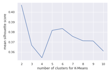
After obtaining the PCA-transformed data, Silhouette Score is implemented to compute the optimal number of clusters to apply in the KMeans approach. The result (Figure 7) shows that a clustering model with 2 clusters performs the best with an average silhouette score of 0.405.
 |
|---|
| Figure 8 |
 |
|---|
| Figure 9 |
To answer the Diabetes Classification question, we apply the XGBoost method to create a decision tree classifier. XGBoost contains a series of hyperparameters. To reach the optimal model without much knowledge regarding the healthcare and insurance industries, we perform the grid search cross-validation of each hyperparameter according to the recommended intervals.
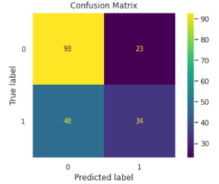
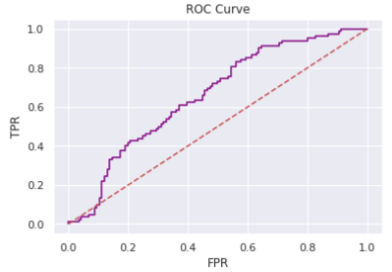
We finalize the model with the following hyperparameters {‘colsample_bytree’: 0.5, ‘gamma’: 0, ‘learning_rate’: 0.01, ‘max_depth’: 7, ‘reg_lambda’: 1, ‘scale_pos_weight’: 1, ‘subsample’: 0.8} with an area under ROC curve value of 0.6511. The following (Figure 10 and Figure 11) shows the result of the optimized classifier.
 |
|---|
| Figure 10 |
 |
|---|
| Figure 11 |
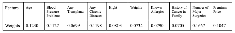
The optimal classifier consists of features with distinct weights shown below.
 |
|---|
| Figure 12 |
From the scatter plot obtained by the KMeans clustering, we see that there exist two groups of people determined by all features except Diabetes which may be used to determine whether or not a person has diabetes. The classification model helps put our assumption to test. However, the area under ROC curve value of 0.6511 implies that our model is not robust enough to corroborate our assumption.
6. Conclusion
- We concluded that age, chronic disease history, and surgery history are factors that affect the insurance premium price.
- Out of three possible regularized regression models (Ridge, LASSO, Elastic net), ridge regression resulted in the highest R2 as well as the lowest RMSE values.
- In the regression model, the “Age” feature had the highest coefficient value, which meant that age had the closest relationship with the premium price.
- Clustering result shows that there exists two potential groups regarding the status of diabetes, however, the classification model does not perform well on determining diabetes patients.
During the analysis, there were few assumptions that were made which could potentially affect the outcome of our analysis. First, we made the assumption that the relationship between the features and the independent variable is linear, but it is very possible that the relationship is non-linear (i.e. polynomial). Also, we made the assumption that the data retrieved for this project had no biased sampling. Particularly, we assumed that there were no other confounding variables which could have impacted the result. Finally, our assumption that these premium prices are of the same insurance plan draws significant limitations to our prediction as different insurance plans offer various coverages, hence, a distinct underlying pricing model for each plan. To mitigate some of the assumptions, we could gather data using stratified sampling, where we create multiple categories or subgroups in which the confounding variables do not vary much, and survey the patients.