Predicting Loan Defaults for Banca Massiccia

Click HERE to see the full and detailed script

Project Overview

This was a project in my Machine Learning in Finance course at NYU. The project aimed at enhancing the bank’s loan underwriting process. Utilizing machine learning, I developed a model to predict the one-year Probability of Default (PD) for prospective borrowers, thereby enabling risk-based pricing and more informed loan decisions.

Workflow

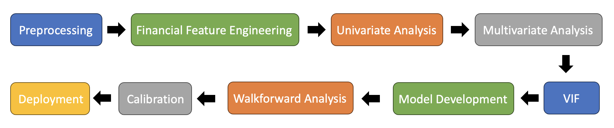
Approach

The approach involved training a logistic regression model on historical bank transaction data. The focus was on key financial indicators to forecast the probability of default for new borrowers.

Techniques

• Feature Engineering: Extracted meaningful indicators such as debt ratio, leverage, and cash return on assets.
• Modeling: Employed logistic regression for default prediction. This was to emphasize explanability of the model.
• Evaluation: Applied finance-specific evaluation methods, including walk-forward testing.

Outcome

The model outputs predicted default probability, which can assist the bank in determining suitable interest rates and underwriting fees. Using the above mentioned techniques, the model’s AUC improved from baseline result of 0.701 to 0.7761.

Usage

Key Files

• estimation.py: This script calculates the AUC of the training dataset, computes the medians of the final variables using the training dataset, and creates model.pkl, the logistic regression model using the final variables.
• harness.py: A consolidating script that inputs the test dataset and outputs predictions. It utilizes model.pkl and prediction.py. In the course, we were not given a test set. If you want to run this model, perhaps use the train data and split into train/test.
• prediction.py: Contains functions for preprocessing the data, running the model on the test dataset, applying calibration, and generating the final output. This gets called in the harness.py.

How to Run

1. Ensure all dependencies are installed.
2. Run estimation.py to train the model and generate model.pkl, along with the parameter values required for the harness.py.
3. Use harness.py with your test dataset to get predictions. This script will call prediction.py for necessary processing and prediction steps.

python3 harness.py --input_csv  <input file in csv> --output_csv <output csv file path to which the predictions are written> 

Data Understanding and Preparation

Problem Formulation

I applied a business-context-aware approach, considering financial factors such as profitability, leverage, and liquidity in our model.

Data Imputation

Handled missing values by replacing them with related financial variables. For example, a variable called roe had some missing values, which were replaced by profit / total equity. After these finance-based imputation, less than 1% of the missing values remained per some variables. These were handled using median imputation.

Engineered Features

• Liquidity: These variables measure the extent to which the firm has liquid assets relative to the size of its liabilities. Æ High liquidity reduces the probability of default. i.e., Time Interest Earned, Current Ratio
• Size: These variables are converted into a common currency as necessary and then are deflated to a specific base year to ensure comparability (e.g., total assets are measured in 2001 U.S. dollars). Æ Large firms default less often. i.e., Total Assets
• Debt Coverage: The ratio of cash flow to interest payments or some other measure of liabilities. Æ High debt coverage reduces the probability of default. i.e.,Leverage Ratio, Debt Ratio
• Profitability: High profitability reduces the probability of default. i.e., Net Profit Margin, Cash Return on Assets
• Activity: These ratios may measure the extent to which a firm has a substantial portion of assets in accounts that may be of subjective value. For example, a firm with a lot of inventories may not be selling its products and may have to write off these inventories. Æ A large stock of inventories relative to sales increases the probability of default; other activity ratios have different relationships to default. i.e., Asset Turnover, Net Working Capital
• Leverage: Leverage refers to the use of debt (borrowed funds) to amplify returns from an investment or project. Higher leverage increases PD. i.e., (Long term debt + Short term debt) / Total Assets

Feature Selection

Baseline Model

A baseline model was developed using a “kitchen sink” approach, where all variables were initially included. This model served as a benchmark for the performance of the refined model. The AUC for this model was 0.701.

Univariate Analysis

• Within the six categories of financial factors, the top (1 to 2) features per financial factors were selected via univariate analysis. This was using a single predictor to predict the target variable (binary column of 1 for is_default and 0 for no_default).
• The variables with the highest AUC score were chosen.

Multivariate Analysis

• While the variable may perform well in the univariate analysis, it is possible that the variable underperforms when other variables are introduced. Therfore, a grid search was conducted using all possible combinations of variables to find the best combinations of variables.
• The combination with the highest AUC score was chosen.

Check Multicollinearity

Logistic Regression is sensitive to multicollinearity. Multicollinearity is when the predictor variables are highly correlated with other predictor variables. As a result, it is hard for the model to estimate the effect of each predictor independently. This can result in unstable coefficients where the signs can be flipped, or become very sensitive to smal lchanges in the model.

Variation Inflation Factor (VIF) was run on the final variables using a threshold of 5 (about 80% of the variance can be explained by other variables), and removed variables that had VIF score of above 5.

Model Evaluation and Interpretation

Walk-Forward Analysis

Implemented walk-forward analysis for a realistic simulation of financial industry behavior, ensuring robust model performance.

Calibration

• Calibration is defined as the process of adjusting the model’s output to make its predictions more accurate and representative of the real world.
• Mapped the Model Output to Match Training Sample Probabilities by using a non-linear curve mapping.

Interpreting Coefficients and P-value

• Verified the coefficients’ signs aligned with our financial understanding, confirming the model’s validity.
• Ensured that variables with p-values under 0.05 were selected as final variables.

Conclusion and Future Work

The final variables used for the model were:

• total asset
• return on asset
• debt ratio
• cash return assets
• leverage

The AUC using these variables was 0.7761. Using financial variables made a significant improvement upon the baseline model (AUC of 0.701).

Further improvements can be made using a more sophisticated models. For example, a non-parameteric tree-based model like XGBoost or Random Forest model can be tested to see the performance of the AUC. Further assessment will be needed to decide if the improvement on AUC is more beneficial than the explainability of the Logistic Regression.